Network Equations and Initial Conditions in Circuit Analysis

Introduction to Network Equations

In circuit analysis, there are two primary methods for writing network equations:

1. Mesh analysis
2. Node analysis

Both methods allow us to solve for unknown currents and voltages in a circuit. The choice between mesh and node analysis often depends on which method requires fewer equations for a given circuit.

Mesh Analysis

Mesh analysis involves identifying closed paths in a circuit called meshes and writing equations based on Kirchhoff's Voltage Law (KVL) for each mesh.

Key Points:

• A mesh is the smallest closed path that does not contain any other closed path within it
• All meshes are loops, but not all loops are meshes
• The number of independent mesh equations required is: B - N + 1 Where B = number of branches, N = number of nodes
• Each circuit element must be included in at least one mesh equation

Example of Mesh Analysis

Let's consider a circuit with two meshes:

     +    L    C1    R1
 e(t) --- ))) ---||--- /\/\/\ ---+
     -                          |
                       C2        |
                      ---||---   |
                               L2 |
                              ))) |
                                  |
                                 R2
                              /\/\/\
                                  |
                                 ---
                                 GND

For this circuit, we would write two mesh equations:

1. For mesh 1 (i1): e(t)u(t) = L(di1/dt) + (1/C1)∫i1dt + R1(i1-i2) + (1/C2)∫(i1-i2)dt

2. For mesh 2 (i2): 0 = L2(di2/dt) + R2i2 + (1/C2)∫(i2-i1)dt + R1(i2-i1)

Node Analysis

Node analysis involves writing equations based on Kirchhoff's Current Law (KCL) for each node in the circuit, except for the reference node (usually ground).

Key Points:

• The number of independent node equations required is: N - 1 Where N = number of nodes
• Node voltages are measured with respect to a reference node

Example of Node Analysis

Consider a circuit with three nodes:

     i(t)u(t)
        |
       R0
        |
    +---+---+
    |       |
   C0      R1
    |       |
    |      L1
    |       |
    +---+---+
        |
       C1
        |
       R2
        |
       GND

For this circuit, we would write three node equations:

1. For node 1 (V1): i(t)u(t) = V1/R0 + C0(dV1/dt) + (V1-V2)/R1 + (1/L)∫(V1-V3)dt

2. For node 2 (V2): 0 = (V2-V1)/R1 + C1(dV2/dt) + V2/R2

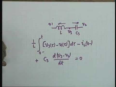
3. For node 3 (V3): 0 = (1/L)∫(V3-V1)dt + C1(d(V3-V2)/dt)

Initial Conditions

When solving differential equations derived from circuit analysis, we need to consider initial conditions. These are typically evaluated at t = 0+, just after a switch is closed or a source is applied.

Methods for Finding Initial Conditions:

1. Physical considerations
2. From the differential equations themselves

Example: RC Circuit

For a simple RC circuit with a voltage source V switched on at t=0:

     +    R
   V --- /\/\/\ ---+
     -             |
                   C
                   |
                  ---
                  GND

• i(0+) = V/R (capacitor acts as a short circuit initially)
• di/dt(0+) = -V/(R^2C) (found by differentiating the circuit equation)

Steady-State Solutions

The steady-state solution is the long-term behavior of the circuit as t approaches infinity. For DC sources, this often involves treating inductors as short circuits and capacitors as open circuits.

Sinusoidal Steady-State

For sinusoidal sources, we can use phasor analysis to find the steady-state solution without solving differential equations.

Example: Current source parallel with RC

   i0sin(ω0t)u(t)
        |
    +---+---+
    |       |
    R       C
    |       |
    +---+---+
        |
       GND

The voltage across the parallel RC combination can be found using phasor analysis:

V(t) = (i0 / √(G^2 + (ω0C)^2)) * sin(ω0t - tan^(-1)(ω0C/G))

Where G = 1/R

Conclusion

Understanding how to write and solve network equations using mesh and node analysis is crucial for circuit analysis. By considering initial conditions and steady-state solutions, engineers can fully describe the behavior of a circuit over time. For sinusoidal sources, phasor analysis provides a powerful tool for finding steady-state solutions without solving complex differential equations.

Article created from: https://youtu.be/gk7HNFBXi_c?si=ONobVY576AjK6lyP